Exploratory research · numerical methods and results
✨ Plasma simulation
Four spherical pulse calculations follow converging hydrogen and CNO mixtures through compression, nuclear burning and expansion. These plots expose the simulated fields and numerical checks behind the ordinary-hydrogen fusion proposal.
Assessment: these are internally consistent one-dimensional burn calculations under prescribed initial conditions. Producing those conditions, retaining a coherent implosion in three dimensions, and validating the radiation model remain consequential open questions. The calculated gains and plant output are conditional on resolving them. This reactor concept has no experimental validation.
Initial conditions · Pulse histories · Numerical checks · Unresolved failure mechanisms · Reproduce the plots
What is being solved
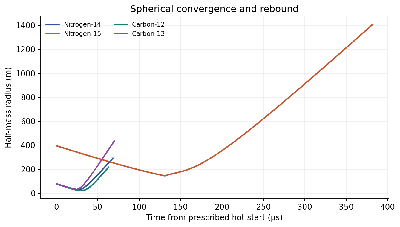
The solver divides a sphere into Lagrangian mass shells. Shell boundaries move under pressure forces, including artificial viscosity for shocks. Cell energy changes through pressure work, nuclear reactions, a modeled weak-energy debit and grey flux-limited radiation diffusion; the same pressure work couples the kinetic and internal energy accounts. A 27-isotope, 194-rate network evolves local abundances. The equation of state combines ideal ions, tabulated electrons and positrons, and radiation in local thermodynamic equilibrium (LTE). The incoming profiles have inward velocities, so the calculation follows their spherical convergence and rebound. The earlier preparation of that inflow is modeled separately and remains a major open problem.
In continuum notation the underlying balances have the forms ∂r/∂t = u, ∂u/∂t = −4πr² ∂(P + q)/∂m, and ∂e/∂t = −(P + q) ∂(1/ρ)/∂t + q̇_nuclear − q̇_weak − ∂L/∂m, with local reaction-network equations for the abundances. Here m is enclosed mass, q is artificial viscosity, and L is radiative luminosity. The q̇ terms are specific energy rates. The center has zero velocity and radiative flux; the outer surface has zero imposed external pressure and an approximate outward radiative flux. The source contains no self-gravity term. The momentum and pressure-work equations use Newtonian bulk dynamics. These equations summarize the model; the implementation defines its discretization and boundary conditions.
The baseline assumes spatially constant grey opacity κ = 0.001 m²/kg. It uses a single material temperature and equilibrium radiation; it does not resolve photon spectra, non-LTE thermalization, separate ion and electron temperatures, magnetic fields or multidimensional flow. Ion Coulomb corrections, nuclear screening and electron conduction are also omitted. The methods note describes the constraints and additional cases.
Selected pulse inputs and outcomes
The selected family uses the actual 128-zone profiles and median carbon-rate update. The time origin is each hot burn's saved initial state. The radius parameter of 30–139.25 m sets the mass and normalization; the actual initial outer radii are 170–888 m. The full radial profiles are in the linked input files. These are separate shots with different masses and starting states.
| Stage | H / catalyst | Mass (kg) | Initial energy (J) | Duration (µs) | Hot gain | Energy residual / input |
|---|---|---|---|---|---|---|
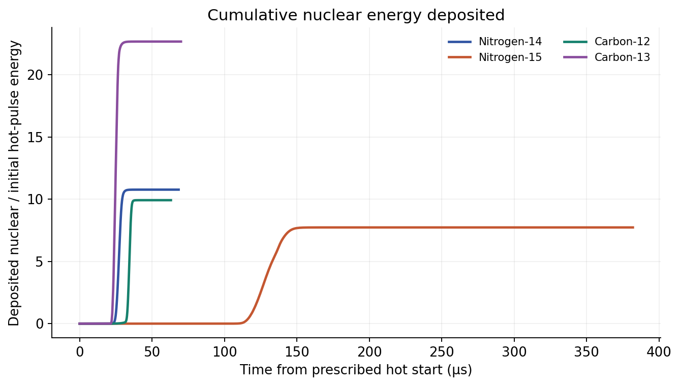
| Nitrogen-14 | 3 | 1.131×10¹³ | 3.493×10²⁵ | 68.395 | 10.765 | −2.68×10⁻⁷ |
| Nitrogen-15 | 2 | 1.131×10¹³ | 3.196×10²⁵ | 381.900 | 7.729 | −1.46×10⁻⁵ |
| Carbon-12 | 2 | 1.131×10¹³ | 4.074×10²⁵ | 63.063 | 9.919 | −3.95×10⁻⁶ |
| Carbon-13 | 2 | 1.131×10¹³ | 3.328×10²⁵ | 70.004 | 22.660 | −2.48×10⁻⁶ |
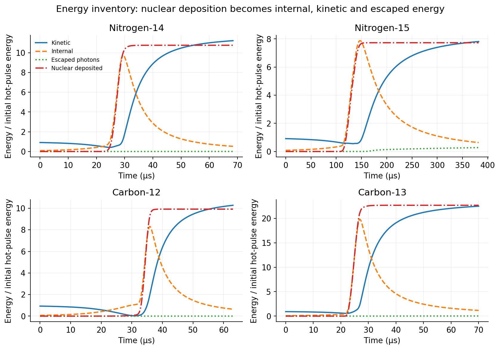
Hot gain is deposited nuclear energy, after the solver's weak-energy debit, divided by initial hot-pulse internal plus kinetic energy. The hot solver assigns the entire positive Q of every weak reaction to escaping energy. This is a conservative hot-heating convention rather than a neutrino-spectrum calculation. Electrical preparation, recovery and auxiliary loads enter the separate plant account. The nitrogen-15 precursor has a slightly higher energy than its hot start because it radiates during preparation; that separate debit is included in the integrated plant account. All four integrations reached their requested end times. The residual compares the final energy ledger with the initial energy; conservation alone does not demonstrate spatial convergence.
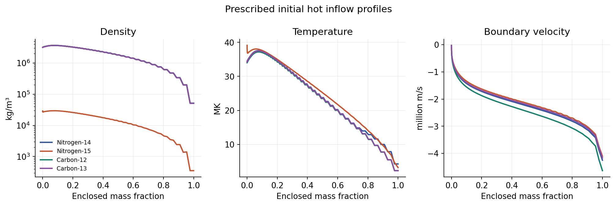
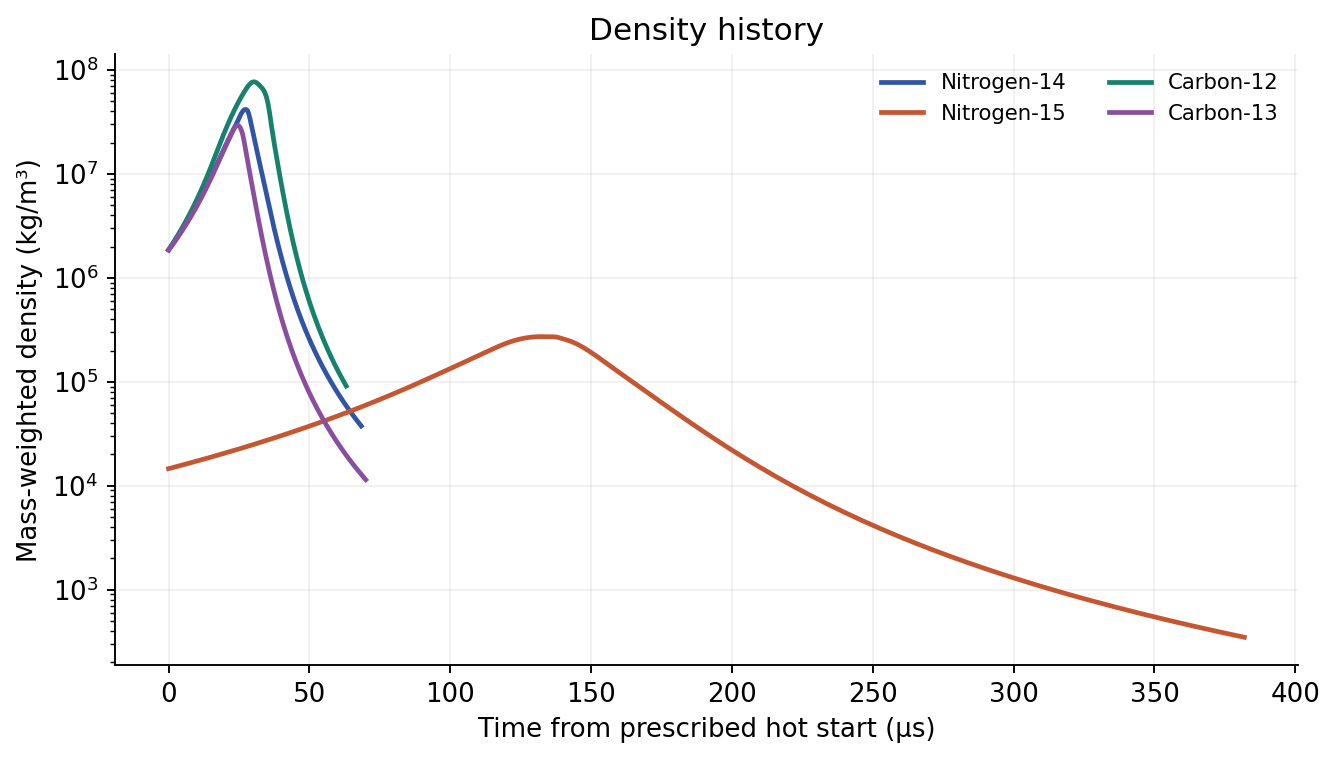
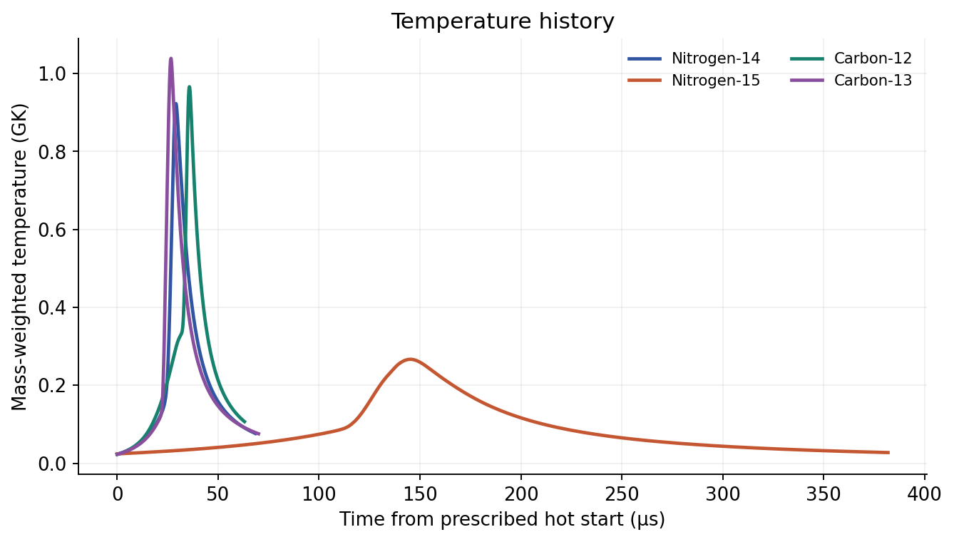
The initial mass-weighted temperatures are 23.1, 24.0, 22.4 and 22.6 million K for N14, N15, C12 and C13. Their mass-weighted densities are 1.85×10⁶, 1.46×10⁴, 1.87×10⁶ and 1.85×10⁶ kg/m³, and their maximum inward boundary speeds are 4.25, 4.11, 4.64 and 4.17 million m/s. About 91–93% of initial energy is bulk kinetic energy. The initial energy denominator includes those reservoirs; a preparation-efficiency assumption does not demonstrate an apparatus capable of producing the spatial profiles.
Pulse histories
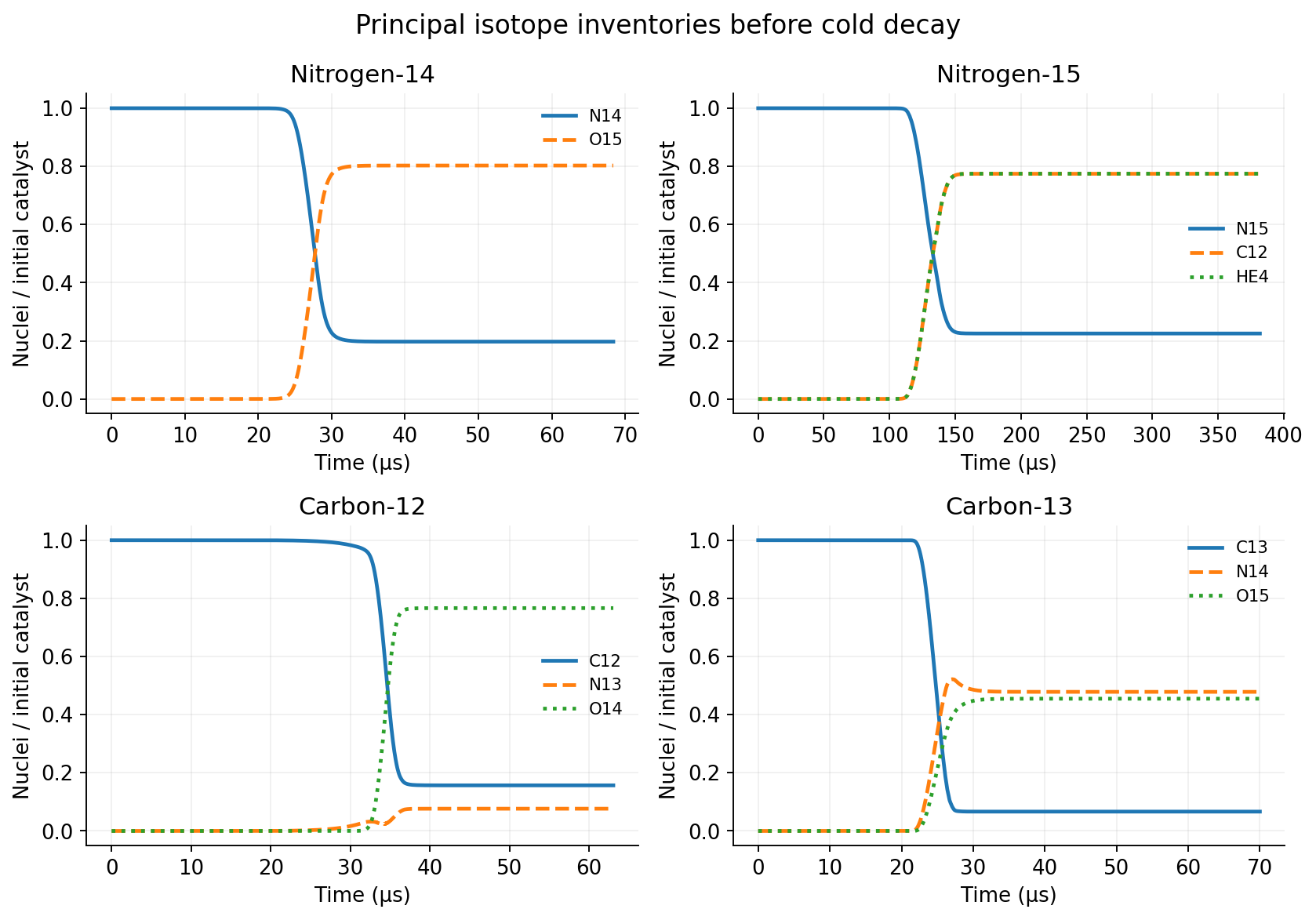
All four curves below use the selected traces. Each contains 400 saved samples; the adaptive integrator takes its own time steps. The samples select accepted solver states by index and have unequal time spacing. Narrow peaks can fall between saved samples. Mass-weighted quantities are ∑mᵢxᵢ/∑mᵢ. Local extrema and volume averages can differ substantially. Each plotted line joins its saved samples. N14 CSV · N15 CSV · C12 CSV · C13 CSV.
Tests and sensitivities
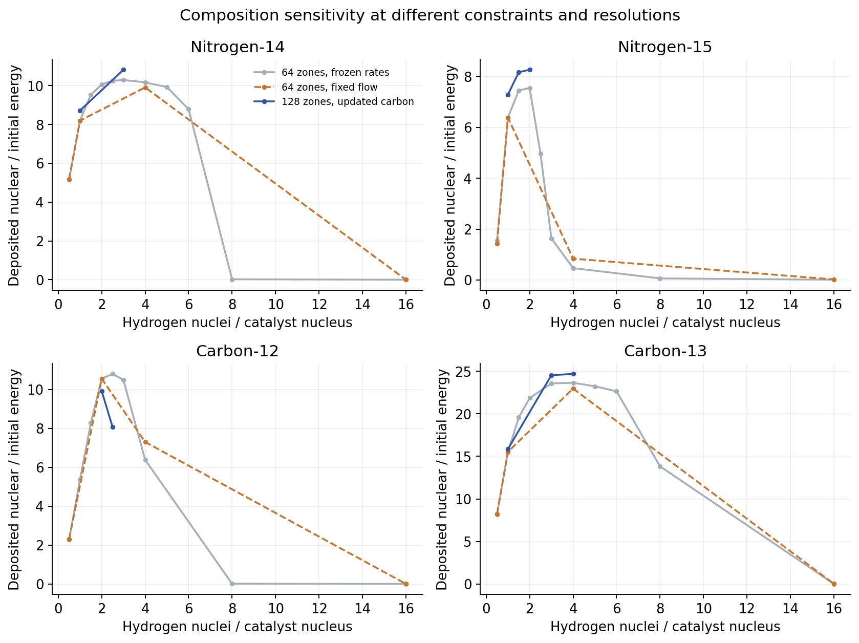
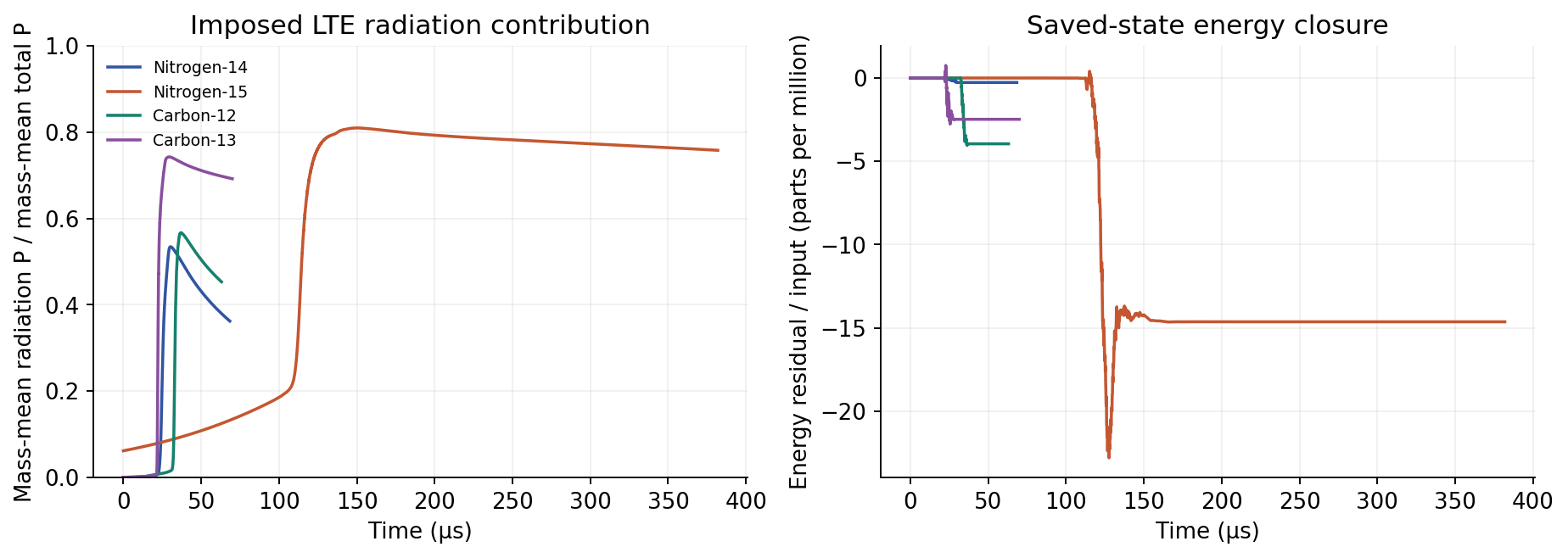
The principal comparison uses relative tolerance 10⁻⁷–10⁻⁶ and absolute tolerance 10⁻¹²–10⁻¹¹, with artificial-viscosity coefficients 0.5 and 2.0. A 2.8 GK numerical/EOS guard terminates incomplete runs, which are excluded from comparisons. The BDF integrator applies those tolerances to normalized state variables. The selected quartet’s endpoint conservation residuals are in the table above.
On the saved states, all four EOS reconstructions remain inside the supplied table’s temperature domain of 10⁵–3×10⁹ K and ρYₑ domain of 10⁻⁶–10⁷ g/cm³. Table coverage establishes interpolation coverage, while physical accuracy requires EOS validation. The underlying electron/positron EOS includes relativistic and degeneracy effects; the bulk hydro remains Newtonian. Saved boundary speeds reach 0.044–0.081c across these cases. Relativistic bulk/radiation-transport corrections have not been quantified for this quartet.
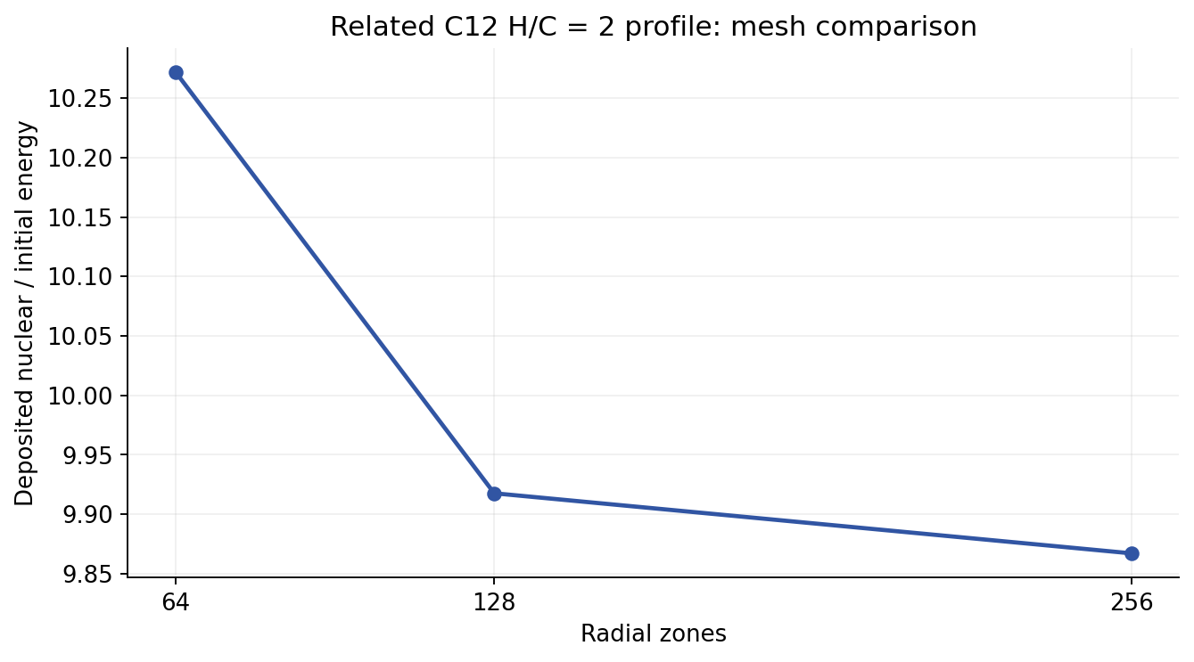
A related quartet gives a nominal 256-cell plant result 0.56% above its 128-cell result, with a longer carbon-return outflow. That comparison retains C13 H/C = 4 and different source profiles; it is supporting evidence rather than convergence of this selected quartet.
The carbon update replaces two proton-capture pairs using the median update associated with the LUNA carbon measurements; the remaining network derives from REACLIB. The implementation applies the same update factor to each forward and reverse pair, preserving the original library equilibrium ratio. This policy is not an independent recalculation of detailed balance from nuclear partition functions. The network includes 27 species up to magnesium and omits deuterium, tritium, helium-3 and carbon-14. The nuclear review documents rate provenance, screening and omitted-channel checks on related histories; it does not qualify every omitted process on these exact final profiles. Rate alternatives, opacity, EOS and source profiles affect results; the tested variations do not provide a comprehensive probability distribution for reactor performance. In particular, the published 80% Monte Carlo interval for the receiver transport reflects sampling at fixed assumptions, not overall reactor uncertainty.
Unresolved failure mechanisms
The fuel assembly simulation follows the nitrogen-15 pulse from pellet release through a conditional merger and burn handoff, with a provisional 90% yield-retention criterion.
The following questions can overturn the claimed reactor performance. The numerical checks above do not answer them.
- Can the prescribed inflow be assembled? The initial profiles already contain dense, multimillion-kelvin fuel with coherent inward momentum. Finite streams, seeds, coatings, neutralization and contact shocks must produce those density, composition, temperature and velocity fields together. A spherical preparation continuation for N15 supplies a model-level construction, while a complete three-dimensional cold-to-burn assembly and its required tolerances remain unverified. Failure here invalidates the operating point even if the hot solver is correct.
- Does radiation actually thermalize on the compression timescale? At each pulse’s peak mass-mean thermodynamic pressure, the imposed LTE radiation contributes 48.3%, 77.1%, 52.5% and 69.4% for N14, N15, C12 and C13. The model sets radiation energy density to aT⁴ and pressure to aT⁴/3 without evolving photon production or a separate radiation temperature. Large grey optical depth alone does not test that closure. Absorption, scattering, spectral transport and matter-radiation equilibration need a coupled calculation on these trajectories. A failure of LTE can change pressure support, temperature and reaction yield.
- Does coherent compression survive perturbations? Spherical symmetry suppresses angular imbalance and mixing. Timing errors, uneven mass loading and finite jets may lower compression or create hotspots and losses. No multidimensional perturbation calculation on this final quartet establishes acceptable launch errors.
- Are yields converged and robust to physics choices? The linked mesh sequence concerns one related profile. A complete resolution, timestep, viscosity and microphysics study of the exact final quartet is still missing. In related N15 calculations, the response to a low reaction-rate curve changes substantially with source profile. The source/rate comparison shows both the weak prescribed-profile case and stronger adjusted-source cases. These demonstrate sensitivity to coupled assumptions rather than a universal tolerance margin.
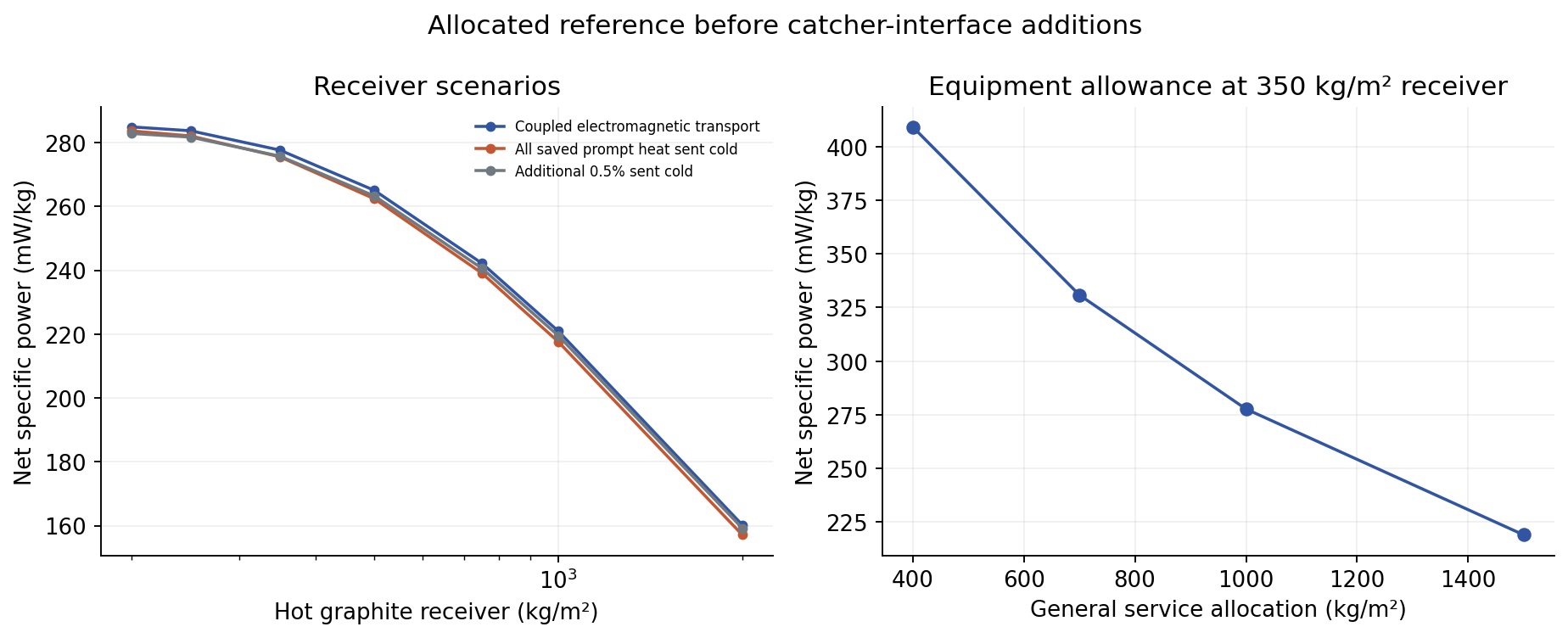
- Does the closed plant retain a useful surplus? Hot-pulse gain precedes driver efficiency, delayed decays, recovery, receiver transport, component replacement and equipment mass. The 277.68 mW/kg result is conditional on those additional accounts. This page’s pulse audit verifies neither their engineering realizability nor a complete component bill.
For the selected runs, photons crossing the plasma surface during the saved interval carry 0.0743%, 7.675%, 0.0191% and 0.1160% of initial-plus-deposited energy for N14, N15, C12 and C13. These fractions follow the assumed grey opacity and LTE closure. They describe the recorded interval; radiation still trapped at its endpoint can escape later. They are not a measurement of total plant heat capture.
Code, data and reproduction
Download the compact reproduction package (code, records, CSVs and input manifest; raw traces downloaded separately). It reproduces all eleven figures with a single driver and creates the output directory. The four original raw traces remain unchanged. Frozen input hashes bind the exact records and EOS table; the original stage map links the quartet to the research archive.
unzip reproduction.zip?v=749f2a4869b4 -d plasma-simulation
cd plasma-simulation
python3.10 -m venv .venv
. .venv/bin/activate
python -m pip install -r code/plot-requirements.txt?v=74bdee5c260e
for stage in n14 n15 c12 c13; do
  curl --fail --location --output "data/$stage.npz" \
    "https://tkwa.me/blog/ordinary-hydrogen-fusion/plasma-simulation/data/$stage.npz"
done
python code/build_plots.py?v=bd7a2ea02878
The tested environment is CPython 3.10.13 with NumPy 1.26.4, SciPy 1.14.0 and Matplotlib 3.9.0. The listed binary versions predate Python 3.14 support. The driver checks input hashes before reduction, trace layout, completion times, masses, initial profiles, endpoint abundances and energy channels. It then regenerates the figures, expanded CSV histories and audit-results.json. The closure calculation uses integrated nuclear energy; the original endpoint residual uses isotope rest-mass changes. Their residuals differ by at most 6×10⁻¹¹ of initial energy for this quartet.
- Unified reduction and plotting code · plot dependencies. The mesh plot reads the supplied comparison records, while the mixture and plant plots read their linked CSVs.
- Original raw traces: N14, N15, C12, C13 (13–14 MB each); data checksums.
- Endpoint / initial profile / inputs: N14 result / initial / inputs; N15 result / initial / inputs; C12 result / initial / inputs; C13 result / initial / inputs. Historical paths in these original records identify research-machine inputs.
- Original hydro, viscosity and radiation implementation; EOS interpolation, actual extended EOS table and table-extension code. The table is derived from pynucastro’s ElectronEOS with ideal ions and LTE radiation.
- Network construction, base rate-library setup, carbon update, carbon-rate table and original simulation dependencies. The input manifest also fingerprints these code snapshots.
- Methods, nuclear review, N15 preparation and burn and four-stage integration are linked at a fixed research-repository revision. The complete design repository contains the broader calculations.
The reproducible step here is reduction of saved runs. A fresh integration of the exact quartet in an independently assembled environment, comparison with an independent hydrodynamics implementation, and experimental validation remain outstanding. Successful plotting and hash checks establish data identity and numerical consistency only.